Parameter Fitting using Spectral Dynamic Causal Modeling

Jupyter Notebook: Please work on DCM.ipynb.

Introduction

Neuroblox provides you with a comprehensive environment for simulations as we have explored previously, but its functionality doesn't stop there. We will now pivot and turn our attention to a different kind of problem: inferring model parameters, that is solving inverse problems, from time series. The method of choice is one of the most widely spread in imaging neuroscience, spectral Dynamic Causal Modeling (spDCM)[1,2]. In this tutorial we will introduce how to perform a spDCM analysis on simulated data. To do so we roughly reproduce the procedure in the SPM script DEM_demo_induced_fMRI.m in Neuroblox. This work was also presented in Hofmann et al.[2]

In this session we will define a circuit of three linear neuronal mass models, all driven by an Ornstein-Uhlenbeck process. We will model fMRI data by a balloon model and BOLD signal on top. After simulation of this simple model we will use spDCM to infer some of the model parameters from the simulation time series.

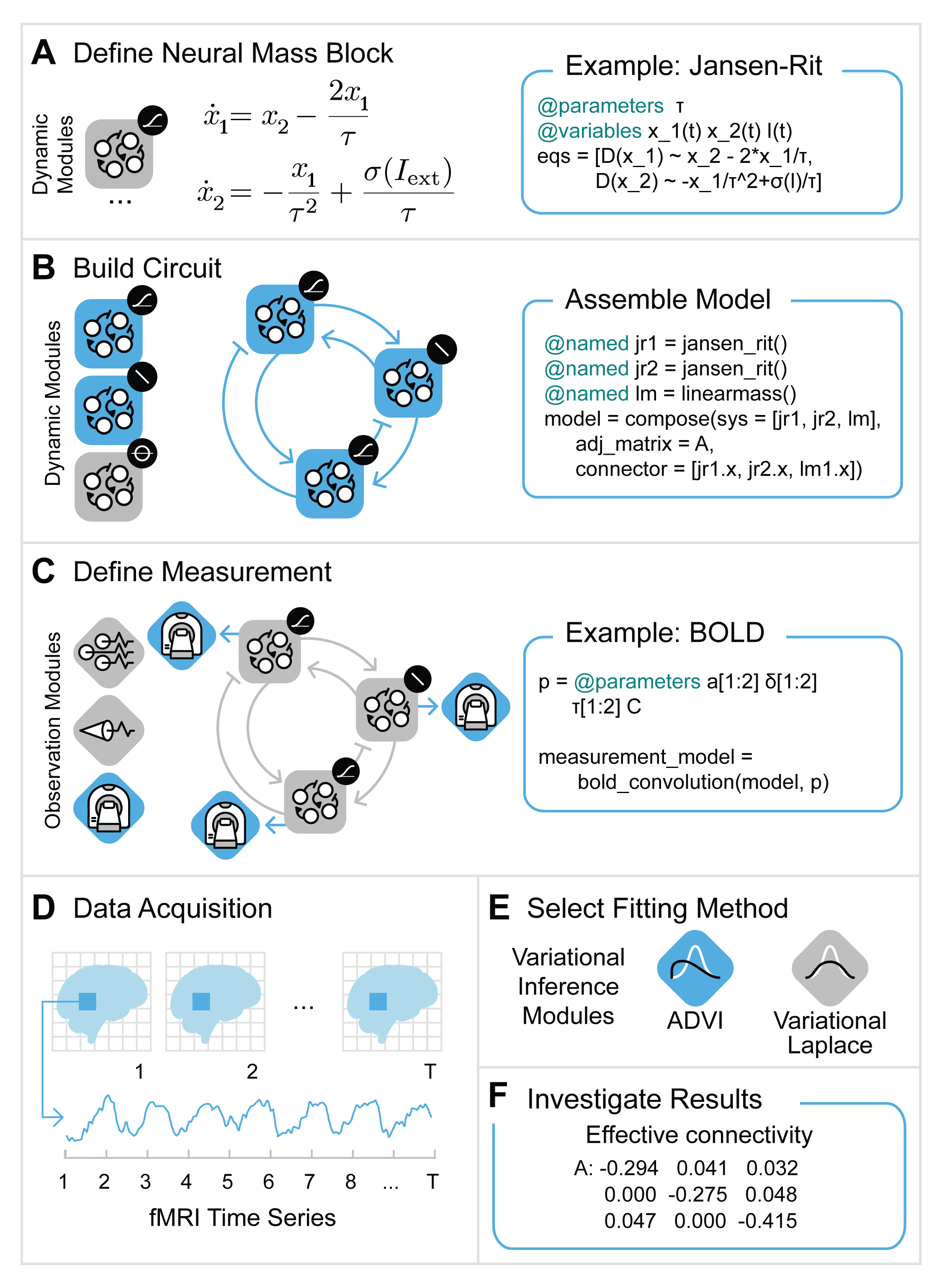Figure 1: Workflow for Spectral DCM analysis.

Figure 1 describes the procedure we will pursue:

• define the graph and add blocks (sections A, B and C in the Figure)

• simulate the model, instead we could also use actual data (section D in Figure)

• compute the cross spectral density

• setup the DCM

• estimate parameters

• plot the results

Learning goals

• perform the entire workflow of an spDCM analysis.

• use observer Blox to simulate experimental measurements.

using Neuroblox
using LinearAlgebra
using StochasticDiffEq
using DataFrames
using OrderedCollections
using CairoMakie
using ModelingToolkit
using Random
using StatsBase

ArgumentError: Package StatsBase not found in current path.
- Run `import Pkg; Pkg.add("StatsBase")` to install the StatsBase package.

Define the model

We will define a model of 3 regions. This means first of all to define a graph. To this graph we will add three linear neuronal mass models which constitute the (hidden) neuronal dynamics. These constitute three nodes of the graph. Next we will also need some input that stimulates the activity, we use simple Ornstein-Uhlenbeck blocks to create stochastic inputs. One per region. We want to simulate fMRI signals thus we will need to also add a BalloonModel per region. Note that the Ornstein-Uhlenbeck block will feed into the linear neural mass which in turn will feed into the BalloonModel blox. This needs to be represented by the way we define the edges.

Random.seed!(17)   # set seed for reproducibility

nr = 3             # number of regions
g = MetaDiGraph()
regions = [];      # list of neural mass blocks to then connect them to each other with an adjacency matrix `A_true`

Now add the different blocks to each region and connect the blocks within each region. For convenience we use a for loop since the type of blocks belonging to a each region repeat over regions but you could also approach building the system the same way as was shown in previous tutorials:

for i = 1:nr
    region = LinearNeuralMass(;name=Symbol("r$(i)₊lm"))
    push!(regions, region)          # store neural mass model in list. We need this list below. If you haven't seen the Julia command `push!` before [see here](http://jlhub.com/julia/manual/en/function/push-exclamation).

    input = OUBlox(;name=Symbol("r$(i)₊ou"), σ=0.2, τ=2)
    add_edge!(g, input => region, weight=1/16)

    measurement = BalloonModel(;name=Symbol("r$(i)₊bm")) ## simulate fMRI signal with BalloonModel which includes the BOLD signal on top of the balloon model dynamics
    add_edge!(g, region => measurement, weight=1.0)
end

Note that weight=1/16 in the connection between the OU process and the Neural Mass Blox is taken from SPM12. This stabilizes the balloon model simulation. Alternatively the noise of the Ornstein-Uhlenbeck block or the weight of the edge connecting neuronal activity and balloon model could be reduced to guarantee numerical stability. Next we define the between-region connectivity matrix and connect regions; we use the same matrix as is defined in [3]

A_true = [[-0.5 -0.2 0]; [0.4 -0.5 -0.3]; [0 0.2 -0.5]]

3×3 Matrix{Float64}:
 -0.5  -0.2   0.0
  0.4  -0.5  -0.3
  0.0   0.2  -0.5

Note that in SPM DCM connection matrices column variables denote output from and rows denote inputs to a particular region. This is different from the usual Neuroblox definition of connection matrices. Thus we flip the indices in what follows:

for idx in CartesianIndices(A_true)
    add_edge!(g, regions[idx[1]] => regions[idx[2]], weight=A_true[idx[2], idx[1]])   # Note the definition of columns as outputs and rows as inputs. For consistency with SPM we keep this notation.
end

finally we compose the simulation model

@named simmodel = system_from_graph(g);

Run the simulation and plot the results

setup simulation of the model, time in seconds

tspan = (0, 1022)
dt = 2   # 2 seconds as measurement interval for fMRI
prob = SDEProblem(simmodel, [], tspan)
sol = solve(prob, ImplicitRKMil(), saveat=dt);

we now want to extract all the variables in our model which carry the tag "measurement". For this purpose we can use the Neuroblox function get_idx_tagged_vars the observable quantity in our model is the BOLD signal, the variable of the Blox BalloonModel that represents the BOLD signal is tagged with "measurement" tag. other tags that are defined are "input" which denotes variables representing a stimulus, like for instance an OUBlox.

idx_m = get_idx_tagged_vars(simmodel, "measurement")    # get index of bold signal

3-element Vector{Int64}:
 19
 20
 21

plot bold signal time series

f = Figure()
ax = Axis(f[1, 1],
    title = "fMRI time series",
    xlabel = "Time [ms]",
    ylabel = "BOLD",
)
lines!(ax, sol, idxs=idx_m)
f

We note that the initial spike is not meaningful and a result of the equilibration of the stochastic process thus we remove it.

dfsol = DataFrame(sol);

Add measurement noise and rescale data

data = Matrix(dfsol[:, idx_m .+ 1]);    # +1 due to the additional time-dimension in the data frame.

add measurement noise

data += randn(size(data))/4;

center and rescale data (as done in SPM):

data .-= mean(data, dims=1);
data *= 1/std(data[:])/4;
dfsol = DataFrame(data, :auto);

UndefVarError: `mean` not defined in `Main.FD_SANDBOX_2630177278844153205`
Suggestion: check for spelling errors or missing imports.
Hint: a global variable of this name may be made accessible by importing Statistics in the current active module Main
Hint: a global variable of this name may be made accessible by importing StatsBase in the current active module Main
Hint: a global variable of this name may be made accessible by importing Distributions in the current active module Main

Add correct names to columns of the data frame

_, obsvars = get_eqidx_tagged_vars(simmodel, "measurement");  # get index of equation of bold state
rename!(dfsol, Symbol.(obsvars))

DimensionMismatch: Length of nms doesn't match length of x.

Estimate and plot the cross-spectral densities

We compute the cross-spectral density by fitting a linear model of order p and then compute the csd analytically from the parameters of the multivariate autoregressive model

p = 8
mar = mar_ml(data, p)   # maximum likelihood estimation of the MAR coefficients and noise covariance matrix
ns = size(data, 1)
freq = range(min(128, ns*dt)^-1, max(8, 2*dt)^-1, 32)
csd = mar2csd(mar, freq, dt^-1);

Now plot the real part of the cross-spectra. Most part of the signal is in the lower frequencies:

fig = Figure(size=(1200, 800))
grid = fig[1, 1] = GridLayout()
for i = 1:nr
    for j = 1:nr
        if i == 1 && j == 1
            ax = Axis(grid[i, j], xlabel="Frequency [Hz]", ylabel="real value of CSD")
        else
            ax = Axis(grid[i, j])
        end
        lines!(ax, freq, real.(csd[:, i, j]))
    end
end
Label(grid[1, 1:3, Top()], "Cross-spectral densities", valign = :bottom,
    font = :bold,
    fontsize = 32,
    padding = (0, 0, 5, 0))
fig

Figure()

These cross-spectral densities are the data we use in spectral DCM to fit our model to and perform the inference of connection strengths.

Model Inference

We will now assemble a new model that is used for fitting the previous simulations. This procedure is similar to before with the difference that we will define global parameters and use tags such as [tunable=false/true] to define which parameters we will want to estimate. Note that parameters are tunable by default.

g = MetaDiGraph()
regions = [];   # list of neural mass blocks to then connect them to each other with an adjacency matrix `A`

Note that parameters are typically defined within a Blox and thus not immediately visible to the user. Since we want some parameters to be shared across several regions we define them outside of the regions. For this purpose use the ModelingToolkit macro @parameters which is used to define symbolic parameters for models. Note that we can set the tunable flag right away thereby defining whether we will include this parameter in the optimization procedure or rather keep it fixed to its predefined value.

@parameters lnκ=0.0 [tunable=false] lnϵ=0.0 [tunable=false] lnτ=0.0 [tunable=false];   # lnκ: decay parameter for hemodynamics; lnϵ: ratio of intra- to extra-vascular components, lnτ: transit time scale
@parameters C=1/16 [tunable=false];   # note that C=1/16 is taken from SPM12 and stabilizes the balloon model simulation. See also comment above.

We now define a similar model as above for the simulation but instead of using an actual stimulus Blox we here add ExternalInput which represents a simple linear external input that is not specified any further. We simply say that our model gets some input with a proportional factor $C$. This is mostly only to make sure that our results are consistent with those produced by SPM

for i = 1:nr
    region = LinearNeuralMass(;name=Symbol("r$(i)₊lm"))
    push!(regions, region)
    input = ExternalInput(;name=Symbol("r$(i)₊ei"))
    add_edge!(g, input => region, weight=C)

    measurement = BalloonModel(;name=Symbol("r$(i)₊bm"), lnτ=lnτ, lnκ=lnκ, lnϵ=lnϵ) ## assume fMRI signal and model them with a BalloonModel
    add_edge!(g, region => measurement, weight=1.0)
end

Here we define the prior expectation values of the effective connectivity matrix we wish to infer:

A_prior = 0.01*randn(nr, nr)
A_prior -= diagm(diag(A_prior))    # remove the diagonal

3×3 Matrix{Float64}:
  0.0         0.0138076   -0.000870584
 -0.0110173   0.0         -0.000945151
 -0.0153045  -0.00676341   0.0

Since we want to optimize these weights we turn them into symbolic parameters: Add the symbolic weights to the edges and connect regions.

A = []
for (i, a) in enumerate(vec(A_prior))
    symb = Symbol("A$(i)")
    push!(A, only(@parameters $symb = a))
end

for (i, idx) in enumerate(CartesianIndices(A_prior))
    if idx[1] == idx[2]
        add_edge!(g, regions[idx[1]] => regions[idx[2]], weight=-exp(A[i])/2)  ## -exp(A[i])/2: treatement of diagonal elements in SPM12 to make diagonal dominance (see Gershgorin Theorem) more likely but it is not guaranteed
    else
        add_edge!(g, regions[idx[2]] => regions[idx[1]], weight=A[i])
    end
end
# Avoid simplification of the model in order to be able to exclude some parameters from fitting
@named fitmodel = system_from_graph(g, simplify=false);

With the function changetune we can provide a dictionary of parameters whose tunable flag should be changed, for instance set to false to exclude them from the optimization procedure. For instance the effective connections that are set to zero in the simulation and the self-connections:

untune = Dict(A[3] => false, A[7] => false, A[1] => false, A[5] => false, A[9] => false)
fitmodel = changetune(fitmodel, untune)           # 3 and 7 are not present in the simulation model
fitmodel = structural_simplify(fitmodel)          # and now simplify the euqations

Model fitmodel:
Equations (21):
  21 standard: see equations(fitmodel)
Unknowns (21): see unknowns(fitmodel)
  r1₊lm₊x(t) [defaults to 0.0]
  r1₊bm₊s(t) [defaults to 0.0]
  r1₊bm₊lnu(t) [defaults to 0.0]
  r1₊bm₊lnν(t) [defaults to 0.0]
  r1₊bm₊lnq(t) [defaults to 0.0]
  r2₊lm₊x(t) [defaults to 0.0]
  r2₊bm₊s(t) [defaults to 0.0]
  r2₊bm₊lnu(t) [defaults to 0.0]
  r2₊bm₊lnν(t) [defaults to 0.0]
  r2₊bm₊lnq(t) [defaults to 0.0]
  r3₊lm₊x(t) [defaults to 0.0]
  r3₊bm₊s(t) [defaults to 0.0]
  r3₊bm₊lnu(t) [defaults to 0.0]
  r3₊bm₊lnν(t) [defaults to 0.0]
  r3₊bm₊lnq(t) [defaults to 0.0]
  r1₊ei₊u(t) [defaults to 0.0]: ext_input
  r2₊ei₊u(t) [defaults to 0.0]: ext_input
  r3₊ei₊u(t) [defaults to 0.0]: ext_input
  r1₊bm₊bold(t) [defaults to 0.0]: measurement
  r2₊bm₊bold(t) [defaults to 0.0]: measurement
  r3₊bm₊bold(t) [defaults to 0.0]: measurement
Parameters (16): see parameters(fitmodel)
  A4 [defaults to 0.0138076]
  A6 [defaults to -0.00676341]
  A8 [defaults to -0.000945151]
  A2 [defaults to -0.0110173]
  C [defaults to 0.0625]
  lnϵ [defaults to 0.0]
  A3 [defaults to -0.0153045]
  A7 [defaults to -0.000870584]
  A1 [defaults to 0.0]
  A5 [defaults to 0.0]
  A9 [defaults to 0.0]
  lnκ [defaults to 0.0]
  lnτ [defaults to 0.0]
  w_r1₊lm_r1₊bm [defaults to 1.0]
  w_r2₊lm_r2₊bm [defaults to 1.0]
  w_r3₊lm_r3₊bm [defaults to 1.0]
Observed (6): see observed(fitmodel)

Setup spectral DCM

max_iter = 128; # maximum number of iterations
# attribute initial conditions or default values to dynamic states of our model
sts, _ = get_dynamic_states(fitmodel);

the following step is needed if the model's Jacobian would give degenerate eigenvalues when expanded around the fixed point 0 (which is the default expansion). We simply add small random values to avoid this degeneracy:

perturbedfp = Dict(sts .=> abs.(10^-10*rand(length(sts))))     # slight noise to avoid issues with Automatic Differentiation.

Dict{SymbolicUtils.BasicSymbolic{Real}, Float64} with 15 entries:
  r3₊lm₊x(t) => 1.10897e-11
  r3₊bm₊lnq(t) => 8.56768e-11
  r2₊bm₊lnq(t) => 4.80233e-11
  r1₊bm₊lnν(t) => 5.27927e-11
  r2₊bm₊s(t) => 6.51909e-11
  r3₊bm₊lnu(t) => 6.74234e-11
  r2₊bm₊lnν(t) => 1.89427e-11
  r1₊bm₊s(t) => 3.51678e-11
  r3₊bm₊lnν(t) => 3.39346e-11
  r1₊lm₊x(t) => 2.54735e-11
  r1₊bm₊lnu(t) => 5.47787e-12
  r3₊bm₊s(t) => 6.77173e-11
  r2₊lm₊x(t) => 6.93896e-11
  r2₊bm₊lnu(t) => 5.51802e-11
  r1₊bm₊lnq(t) => 7.86157e-11

For convenience we can use the default prior function to use standardized prior values as given in SPM:

pmean, pcovariance, indices = defaultprior(fitmodel, nr)

priors = (μθ_pr = pmean,
          Σθ_pr = pcovariance
         );

Setup hyper parameter prior as well:

hyperpriors = Dict(:Πλ_pr => 128.0*ones(1, 1),   # prior metaparameter precision, needs to be a matrix
                   :μλ_pr => [8.0]               # prior metaparameter mean, needs to be a vector
                  );

To compute the cross spectral densities we need to provide the sampling interval of the time series, the frequency axis and the order of the multivariate autoregressive model:

csdsetup = (mar_order = p, freq = freq, dt = dt);

Prepare the DCM. This function will setup the computation of the Dynamic Causal Model. The last parameter specifies that we are using fMRI time series (as opposed to LFPs, which is the other modality that is currently available in Neuroblox).

(state, setup) = setup_sDCM(dfsol, fitmodel, perturbedfp, csdsetup, priors, hyperpriors, indices, pmean, "fMRI");

type Dict has no field μλ_pr

We are now ready to run the optimization procedure! That is we loop over runsDCMiteration! which will alter state after each optimization iteration. It essentially computes the Variational Laplace estimation of expectation and variance of the tunable parameters.

for iter in 1:max_iter
    state.iter = iter
    run_sDCM_iteration!(state, setup)
    print("iteration: ", iter, " - F:", state.F[end], " - dF predicted:", state.dF[end], "\n")
    if iter >= 4
        criterion = state.dF[end-3:end] .< setup.tolerance
        if all(criterion)
            print("convergence\n")
            break
        end
    end
end

UndefVarError: `state` not defined in `Main.FD_SANDBOX_2630177278844153205`
Suggestion: check for spelling errors or missing imports.

Note that the output F is the free energy at each iteration step and dF is the predicted change of free energy at each step which approximates the actual free energy change and is used as stopping criterion by requiring that it does not excede the tolerance level for 4 consecutive times.

Results

Free energy is the objective function of the optimization scheme of spectral DCM. Note that in the machine learning literature this it is called Evidence Lower Bound (ELBO). Plot the free energy evolution over optimization iterations to see how the algorithm converges towards a (potentially local) optimum:

f1 = freeenergy(state)

UndefVarError: `state` not defined in `Main.FD_SANDBOX_2630177278844153205`
Suggestion: check for spelling errors or missing imports.

// Image matching '/assets/pages/DCM/code/freeenergy' not found. //

Plot the estimated posterior of the effective connectivity and compare that to the true parameter values. Bar height are the posterior mean and error bars are the standard deviation of the posterior.

f2 = ecbarplot(state, setup, A_true)

UndefVarError: `state` not defined in `Main.FD_SANDBOX_2630177278844153205`
Suggestion: check for spelling errors or missing imports.

// Image matching '/assets/pages/DCM/code/ecbar' not found. //

Challenge Problems

• Explore susceptibility with respect to noise. Run the script again with a different random seed and observe how the results change. Given that we didn’t change any parameters of the ground truth, what is your take on parameter inference with this setup? How reliable is model selection based on free energy (compare the different free energies of the models and their respective parameter values with ground truth)?

• Averaging over patients. Now repeat the simulation and inference again with 10 different seeds (you can just remove the number in Random.seed() to use current time stamps as seeds) and store the results of each run, such that you get several models based on the same ground truth but with different instances of the noise. Can you extract the average value of the effective connectivity from the ensemble?

• Changing neuronal dynamics model. Now change the model and test the whole procedure with a different underlying neuronal mass model, for instance the Jansen-Rit model. Note that there are no default priors for the Jansen-Rit model, you will have to provide priors for the extra parameters or remove them from the optimization procedure by setting their tunable to false.

References

• [1] Novelli, Leonardo, Karl Friston, and Adeel Razi. “Spectral Dynamic Causal Modeling: A Didactic Introduction and Its Relationship with Functional Connectivity.” Network Neuroscience 8, no. 1 (April 1, 2024): 178–202.
  

• [2] Hofmann, David, Anthony G. Chesebro, Chris Rackauckas, Lilianne R. Mujica-Parodi, Karl J. Friston, Alan Edelman, and Helmut H. Strey. “Leveraging Julia’s Automated Differentiation and Symbolic Computation to Increase Spectral DCM Flexibility and Speed.” bioRxiv: The Preprint Server for Biology, 2023.
  

• [3] Friston, Karl J., Joshua Kahan, Bharat Biswal, and Adeel Razi. “A DCM for Resting State fMRI.” NeuroImage 94 (July 2014): 396–407.

References

CC BY-SA 4.0 Neuroblox Inc. Last modified: July 22, 2025.
Website built with Franklin.jl and the Julia programming language.