Getting Started
Getting Started with Julia
Here we would like to summarize some resources for people that are interested in learning more about the Julia language before or while exploring Neuroblox. Please follow the links below for introductory material on the language that is inclusive to all users; people familiar with programming or not, people with a mathematics, engineering, or science background :
- Introduction to Julia by Matt Bauman at the JuliaCon 2024
- Julia Tutorials & Workshops, a collection of training materials from the official Julia website.
- Modern Julia Workflows, an introduction to how to write and share your Julia code effectively with tips & tricks.
Getting Started with Neuroblox
Overview of the Neuroblox Ecosystem
Neuroblox is organized into several levels of abstraction to support a wide range of modeling needs:
- Low-level (single neurons): Individual neuron models (e.g., Hodgkin-Huxley neurons) that simulate the membrane voltage and ionic currents of a single cell.
- Mid-level (neural masses / populations): Models like Wilson-Cowan or Jansen-Rit that represent the average activity of an entire population of neurons as a compact set of differential equations. These are useful for modeling brain regions and large-scale dynamics.
- Composite blocks: Higher-level structures (e.g.,
WinnerTakeAll,Cortical) that bundle multiple neurons or neural masses into reusable circuit motifs. - Utility functions: Functions for extracting simulation results (
state_timeseries,voltage_timeseries), computing power spectra, plotting raster plots, and more.
Throughout the tutorials you will encounter all of these levels, building from individual neurons up to whole-brain circuits. This tutorial starts at the mid-level with a neural mass model to get you running simulations quickly.
This example will introduce you to simulating brain dynamics using Neuroblox. We will create a simple oscillating circuit using two Wilson-Cowan neural mass models [1]. The Wilson-Cowan model is one of the most influential models in computational neuroscience [2], describing the dynamics of interactions between populations of excitatory and inhibitory neurons.
The Wilson-Cowan Model
Each Wilson-Cowan neural mass is described by the following equations:
\[\begin{align} \nonumber \frac{dE}{dt} &= \frac{-E}{\tau_E} + S_E(c_{EE}E - c_{IE}I + \eta\textstyle\sum{jcn})\\[10pt] \nonumber \frac{dI}{dt} &= \frac{-I}{\tau_I} + S_I\left(c_{EI}E - c_{II}I\right) \end{align}\]
where $E$ and $I$ denote the activity levels of the excitatory and inhibitory populations, respectively. The terms $\frac{dE}{dt}$ and $\frac{dI}{dt}$ describe the rate of change of these activity levels over time. The parameters $\tau_E$ and $\tau_I$ are time constants analogous to membrane time constants in single neuron models, determining how quickly the excitatory and inhibitory populations respond to changes. The coefficients $c_{EE}$ and $c_{II}$ represent self-interaction (or feedback) within excitatory and inhibitory populations, while $c_{IE}$ and $c_{EI}$ represent the cross-interactions between the two populations. The term $\eta\sum{jcn}$ represents external input to the excitatory population from other brain regions or external stimuli, with $\eta$ acting as a scaling factor. While $S_E$ and $S_I$ are sigmoid functions that represent the responses of neuronal populations to input stimuli, defined as:
\[S_k(x) = \frac{1}{1 + exp(-a_kx - \theta_k)}\]
where $a_k$ and $\theta_k$ determine the steepness and threshold of the response, respectively.
Building the Circuit
Let's create an oscillating circuit by connecting two Wilson-Cowan neural masses:
using Neuroblox
using OrdinaryDiffEqRosenbrock
using CairoMakie

# Create a graph of two Wilson-Cowan blox to represent our circuit
@graph g begin
    @nodes begin
        WC1 = WilsonCowan()
        WC2 = WilsonCowan()
    end
    @connections begin
        WC1 => WC1, (weight = -1) ## recurrent connection from WC1 to itself
        WC1 => WC2, (weight =  7) ## connection from WC1 to WC2
        WC2 => WC1, (weight =  4) ## connection from WC2 to WC1
        WC2 => WC2, (weight = -1) ## recurrent connection from WC2 to itself
    end
end
GraphSystem(...2 nodes and 4 connections...)Here, we've created two Wilson-Cowan blox and connected them as nodes in a directed graph. Each blox connects to itself and to the other blox.
By default, the output of each Wilson-Cowan blox is its excitatory activity (E). The negative self-connections (-1) provide inhibitory feedback, while the positive inter-blox connections (6) provide strong excitatory coupling. This setup creates an oscillatory dynamic between the two Wilson-Cowan units.
Creating the Model
Now, let's build the complete model:
prob = ODEProblem(g, [], (0.0, 100), [])ODEProblem with uType Vector{Float64} and tType Float64. In-place: true
Non-trivial mass matrix: false
timespan: (0.0, 100.0)
u0: 4-element Vector{Float64}:
1.0
1.0
1.0
1.0This creates an efficient differential equations system from our graph representation using GraphDynamics.
Simulating the Model
We are now ready to simulate our model. The following code solvesthe ODEProblem for our system, simulating 100 time units of activity. In Neuroblox, the default time unit is milliseconds. We use Rodas4, a solver efficient for stiff problems. The solution is saved every 0.1 ms, allowing us to observe the detailed evolution of the system's behavior.
sol = solve(prob, Rodas4(), saveat=0.1)retcode: Success
Interpolation: 1st order linear
t: 1001-element Vector{Float64}:
0.0
0.1
0.2
0.3
0.4
0.5
0.6
0.7
0.8
0.9
⋮
99.2
99.3
99.4
99.5
99.6
99.7
99.8
99.9
100.0
u: 1001-element Vector{Vector{Float64}}:
[1.0, 1.0, 1.0, 1.0]
[0.9493257635566694, 0.999997227549365, 0.9968352574060094, 0.9999983614072379]
[0.8972980729622233, 0.9999897131895668, 0.9922642579108254, 0.9999967482029593]
[0.8440391811260224, 0.9999681723259077, 0.9854388758920339, 0.999995076307697]
[0.7898349351204718, 0.9999082303969463, 0.9750726533220467, 0.9999931987811771]
[0.7351468545581609, 0.9997317040527284, 0.9591819783728336, 0.9999908111737857]
[0.6805567621145077, 0.999147043910833, 0.9353051118230763, 0.9999870244686659]
[0.6267161119059087, 0.9976995169055252, 0.9005839696994439, 0.9999806570867977]
[0.5745445542719343, 0.9931773367150695, 0.8545965249945568, 0.9999637048536514]
[0.5248014014381632, 0.9822251893286915, 0.7986897069764031, 0.9999118449047143]
⋮
[0.2827951847640496, 0.23241952852966843, 0.31706361763697477, 0.3471838455135568]
[0.2781779459256137, 0.22328371239125663, 0.31279792715965477, 0.33322610439312456]
[0.274480886542364, 0.2143053998661904, 0.3098099262690292, 0.319915421962287]
[0.2718187834280029, 0.205673510137564, 0.30820728524811597, 0.30756838705022216]
[0.2702755782307122, 0.19759133790122987, 0.3080567597540317, 0.2965051666684053]
[0.2698099045024102, 0.19023716779344785, 0.30928326784170707, 0.28692620357578746]
[0.27050297529084105, 0.18373150936886548, 0.3119234621138225, 0.2790718675463413]
[0.2723876533299345, 0.17825467421576754, 0.31592226257658107, 0.27326609552613773]
[0.2754968013536197, 0.17398697392244233, 0.32122458923618413, 0.26983282446125184]Plotting simulation results
Finally, let us plot the E and I states of the first component, WC1. Neuroblox provides a family of functions for extracting simulation results from a solution object. state_timeseries(blox, sol, state_name) is the general-purpose version: given a blox and a solved ODE solution, it returns the time series of the named state variable as a plain Julia vector. Here we use it to extract the excitatory (E) and inhibitory (I) activity of WC1.
E1 = state_timeseries(WC1, sol, "E")
I1 = state_timeseries(WC1, sol, "I")

fig = Figure()
ax = Axis(fig[1,1]; xlabel = "time (ms)")
lines!(ax, sol.t, E1, label = "E")
lines!(ax, sol.t, I1, label = "I")
Legend(fig[1,2], ax)
fig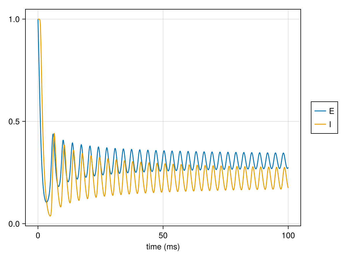
This page was generated using Literate.jl.